Related Definitions
Random variable: It is not a variable in the traditional sense of the world. It is actually a function. The outcome of an experiment need not be a number, for example, the outcome when a coin is tossed can be 'heads' or 'tails'. However, we often want to represent outcomes as numbers [STEPS]. A random variable is a function that associates a unique numerical value with every outcome of an experiment. Random variable is written as capital letter, usually X.
Probability distribution and probability density are similar, where distribution is used for discrete variable and density is used for continuous variable.
Expected Value: The expected value (or population mean) of a random variable indicates its average or central value. It is a useful summary value (a number) of the variable's distribution [STEPS].
The expected value of a random variable X is symbolised by E(X) or µ.
If X is a discrete random variable with possible values x1, x2, x3, ..., xn, and p(xi) denotes P(X = xi), then the expected value of X is defined by:

where the elements are summed over all values of the random variable X.
If X is a continuous random variable with probability density function f(x), then the expected value of X is defined by:

Example:
Discrete case : When a die is thrown, each of the possible faces 1, 2, 3, 4, 5, 6 (the xi's) has a probability of 1/6 (the p(xi)'s) of showing. The expected value of the face showing is therefore:
µ = E(X) = (1 x 1/6) + (2 x 1/6) + (3 x 1/6) + (4 x 1/6) + (5 x 1/6) + (6 x 1/6) = 3.5
Notice that, in this case, E(X) is 3.5, which is not a possible value of X.
Probability Distribution: The probability distribution of a discrete random variable is a list of probabilities associated with each of its possible values. It is also sometimes called the probability function or the probability mass function [STEPS].
More formally, the probability distribution of a discrete random variable X is a function which gives the probability p(xi) that the random variable equals xi, for each value xi:
p(xi) = P(X = xi)
It satisfies the following conditions:


Multivalued Function: A multivalued function, also known as a multiple-valued function (Knopp 1996, part 1 p. 103), is a "function" that assumes two or more distinct values in its range for at least one point in its domain. While these "functions" are not functions in the normal sense of being one-to-one or many-to-one, the usage is so common that there is no way to dislodge it. When considering multivalued functions, it is therefore necessary to refer to usual "functions" as single-valued functions [Wikipedia].
Multivalued Function is also known as: multifunction, many-valued function, set-valued function, set-valued map, point-to-set map, multi-valued map, multimap, correspondence, carrier
While the trigonometric, hyperbolic, exponential, and integer power functions are all single-valued functions, their inverses are multivalued.
Set-Valued Map: Let X and Y be topological spaces. If for each x ∈ X there is a corresponding set F(x) ⊂ Y , then F(·) is called a set-valued map from X to Y . We denote this by
F : X → 2^Y
Set-valued analysis: Instead of considering collections of only points, set-valued analysis considers collections of sets.
Dempster–Shafer Theory (DST)
The theory of belief functions, also referred to as evidence theory or Dempster–Shafer theory (DST), is a well established general framework for reasoning with uncertainty, with understood connections to other frameworks such as probability, possibility and imprecise probability theories [Wikipedia].
The theory allows one to combine evidence from different sources and arrive at a degree of belief (represented by a mathematical object called belief function) that takes into account all the available evidence.
Often used as a method of sensor fusion, Dempster–Shafer theory is based on two ideas: obtaining degrees of belief for one question from subjective probabilities for a related question, and Dempster's rule[1] for combining such degrees of belief when they are based on independent items of evidence. In essence, the degree of belief in a proposition depends primarily upon the number of answers (to the related questions) containing the proposition, and the subjective probability of each answer.
Dempster–Shafer theory assigns its masses to all of the non-empty subsets of the propositions that compose a system. (In set-theoretic terms, the Power set of the propositions.) For instance, assume a situation where there are two related questions, or propositions, in a system. In this system, any belief function assigns mass to the first proposition, the second, both or neither.
Belief and Plausibility: Shafer's framework allows for belief about a propositions to be represented as intervals, bounded by two values, belief (or support) and plausibility:
belief ≤ plausibility.
In a first step, subjective probabilities (masses) are assigned to all subsets of the frame; usually, only a restricted number of sets will have non-zero mass (focal elements).[2]:39f. Belief in a hypothesis is constituted by the sum of the masses of all sets enclosed by it. It is the amount of belief that directly supports a given hypothesis or a more specific one, forming a lower bound. Belief (usually denoted Bel) measures the strength of the evidence in favor of a proposition p. It ranges from 0 (indicating no evidence) to 1 (denoting certainty). It is also known as lower probability.
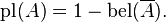
Plausibility (a.k.a., upper probability) is 1 minus the sum of the masses of all sets whose intersection with the hypothesis is empty. Or it can be obtained as the sum of the masses of all sets whose intersection with the hypothesis is not empty. It is an upper bound on the possibility that the hypothesis could be true, i.e. it “could possibly be the true state of the system” up to that value, because there is only so much evidence that contradicts that hypothesis. Plausibility (denoted by Pl) is defined to be Pl(p)=1-Bel(~p). It also ranges from 0 to 1 and measures the extent to which evidence in favor of ~p leaves room for belief in p.
For example, suppose we have a belief of 0.5 and a plausibility of 0.8 for a proposition, say “the cat in the box is dead.” This means that we have evidence that allows us to state strongly that the proposition is true with a confidence of 0.5. However, the evidence contrary to that hypothesis (i.e. “the cat is alive”) only has a confidence of 0.2. The remaining mass of 0.3 (the gap between the 0.5 supporting evidence on the one hand, and the 0.2 contrary evidence on the other) is “indeterminate,” meaning that the cat could either be dead or alive. This interval represents the level of uncertainty based on the evidence in your system.
The null hypothesis is set to zero by definition (it corresponds to “no solution”). The orthogonal hypotheses “Alive” and “Dead” have probabilities of 0.2 and 0.5, respectively. This could correspond to “Live/Dead Cat Detector” signals, which have respective reliabilities of 0.2 and 0.5. Finally, the all-encompassing “Either” hypothesis (which simply acknowledges there is a cat in the box) picks up the slack so that the sum of the masses is 1. The belief for the “Alive” and “Dead” hypotheses matches their corresponding masses because they have no subsets; belief for “Either” consists of the sum of all three masses (Either, Alive, and Dead) because “Alive” and “Dead” are each subsets of “Either”. The “Alive” plausibility is 1 − m (Dead) and the “Dead” plausibility is 1 − m (Alive). In other words, the “Alive” plausibility is m(Alive) + m (Either) and the “Dead” plausibility is m(Dead) + m(Either). Finally, the “Either” plausibility sums m(Alive) + m(Dead) + m(Either). The universal hypothesis (“Either”) will always have 100% belief and plausibility —it acts as a checksum of sorts.
Here is a somewhat more elaborate example where the behavior of belief and plausibility begins to emerge. Suppose we're looking through a variety of detector systems at a single faraway signal light, which can only be coloured in one of three colours (red, yellow, or green):
The event "Red or Yellow" would be considered as the union of the events "Red" and "Yellow", and (see probability axioms) P(Red or Yellow) ≥ P(Yellow), and P(Any)=1, where Any refers to Red or Yellow or Green. In DST the mass assigned to Any refers to the proportion of evidence that can't be assigned to any of the other states, which here means evidence that says there is a light but doesn't say anything about what color it is.
In this example, the proportion of evidence that shows the light is either Red or Green is given a mass of 0.05. Such evidence might, for example, be obtained from a R/G color blind person. DST lets us extract the value of this sensor's evidence. Also, in DST the Null set is considered to have zero mass, meaning here that the signal light system exists and we are examining its possible states, not speculating as to whether it exists at all.
Formal Definition: Let X be the universe: the set representing all possible states of a system under consideration. The power set

is the set of all subsets of X, including the empty set the . For example, if:

then
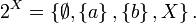
The elements of the power set can be taken to represent propositions concerning the actual state of the system, by containing all and only the states in which the proposition is true.
The theory of evidence assigns a belief mass to each element of the power set. Formally, a function
![m: 2^X \rightarrow [0,1] \,\!](http://upload.wikimedia.org/math/5/1/9/5192b7f90e5798aabb013dcce441e4e2.png)
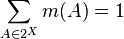
is called a basic belief assignment (BBA), when it has two properties. First, the mass of the empty set is zero:

Second, the masses of the remaining members of the power set add up to a total of 1:
The mass m(A) of A, a given member of the power set, expresses the proportion of all relevant and available evidence that supports the claim that the actual state belongs to A but to no particular subset of A. The value of m(A) pertains only to the set A and makes no additional claims about any subsets of A, each of which have, by definition, their own mass.
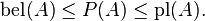
From the mass assignments, the upper and lower bounds of a probability interval can be defined. This interval contains the precise probability of a set of interest (in the classical sense), and is bounded by two non-additive continuous measures called belief (or support) and plausibility:
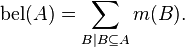
The belief bel(A) for a set A is defined as the sum of all the masses of subsets of the set of interest:
The plausibility pl(A) is the sum of all the masses of the sets B that intersect the set of interest A:
The two measures are related to each other as follows:
For example, suppose we have a belief of 0.5 and a plausibility of 0.8 for a proposition, say “the cat in the box is dead.” This means that we have evidence that allows us to state strongly that the proposition is true with a confidence of 0.5. However, the evidence contrary to that hypothesis (i.e. “the cat is alive”) only has a confidence of 0.2. The remaining mass of 0.3 (the gap between the 0.5 supporting evidence on the one hand, and the 0.2 contrary evidence on the other) is “indeterminate,” meaning that the cat could either be dead or alive. This interval represents the level of uncertainty based on the evidence in your system.
| Hypothesis | Mass | Belief | Plausibility |
|---|---|---|---|
| Null (neither alive nor dead) | 0 | 0 | 0 |
| Alive | 0.2 | 0.2 | 0.5 |
| Dead | 0.5 | 0.5 | 0.8 |
| Either (alive or dead) | 0.3 | 1.0 | 1.0 |
The null hypothesis is set to zero by definition (it corresponds to “no solution”). The orthogonal hypotheses “Alive” and “Dead” have probabilities of 0.2 and 0.5, respectively. This could correspond to “Live/Dead Cat Detector” signals, which have respective reliabilities of 0.2 and 0.5. Finally, the all-encompassing “Either” hypothesis (which simply acknowledges there is a cat in the box) picks up the slack so that the sum of the masses is 1. The belief for the “Alive” and “Dead” hypotheses matches their corresponding masses because they have no subsets; belief for “Either” consists of the sum of all three masses (Either, Alive, and Dead) because “Alive” and “Dead” are each subsets of “Either”. The “Alive” plausibility is 1 − m (Dead) and the “Dead” plausibility is 1 − m (Alive). In other words, the “Alive” plausibility is m(Alive) + m (Either) and the “Dead” plausibility is m(Dead) + m(Either). Finally, the “Either” plausibility sums m(Alive) + m(Dead) + m(Either). The universal hypothesis (“Either”) will always have 100% belief and plausibility —it acts as a checksum of sorts.
Here is a somewhat more elaborate example where the behavior of belief and plausibility begins to emerge. Suppose we're looking through a variety of detector systems at a single faraway signal light, which can only be coloured in one of three colours (red, yellow, or green):
| Hypothesis | Mass | Belief | Plausibility |
|---|---|---|---|
| Null | 0 | 0 | 0 |
| Red | 0.35 | 0.35 | 0.56 |
| Yellow | 0.25 | 0.25 | 0.45 |
| Green | 0.15 | 0.15 | 0.34 |
| Red or Yellow | 0.06 | 0.66 | 0.85 |
| Red or Green | 0.05 | 0.55 | 0.75 |
| Yellow or Green | 0.04 | 0.44 | 0.65 |
| Any | 0.1 | 1.0 | 1.0 |
In this example, the proportion of evidence that shows the light is either Red or Green is given a mass of 0.05. Such evidence might, for example, be obtained from a R/G color blind person. DST lets us extract the value of this sensor's evidence. Also, in DST the Null set is considered to have zero mass, meaning here that the signal light system exists and we are examining its possible states, not speculating as to whether it exists at all.
Formal Definition: Let X be the universe: the set representing all possible states of a system under consideration. The power set
is the set of all subsets of X, including the empty set the
. For example, if:then
The elements of the power set can be taken to represent propositions concerning the actual state of the system, by containing all and only the states in which the proposition is true.
The theory of evidence assigns a belief mass to each element of the power set. Formally, a function
is called a basic belief assignment (BBA), when it has two properties. First, the mass of the empty set is zero:
Second, the masses of the remaining members of the power set add up to a total of 1:
The mass m(A) of A, a given member of the power set, expresses the proportion of all relevant and available evidence that supports the claim that the actual state belongs to A but to no particular subset of A. The value of m(A) pertains only to the set A and makes no additional claims about any subsets of A, each of which have, by definition, their own mass.
From the mass assignments, the upper and lower bounds of a probability interval can be defined. This interval contains the precise probability of a set of interest (in the classical sense), and is bounded by two non-additive continuous measures called belief (or support) and plausibility:
The belief bel(A) for a set A is defined as the sum of all the masses of subsets of the set of interest:
The plausibility pl(A) is the sum of all the masses of the sets B that intersect the set of interest A:
The two measures are related to each other as follows:
Random Set
A random set is a multivalued measurable function defined on a probability space. It serves mainly as a rigorous machinery for modeling observed phenomena which are sets rather than precise points [Scholarpedia].
References:
[1] Dempster, Arthur P.; A generalization of Bayesian inference, Journal of the Royal Statistical Society, Series B, Vol. 30, pp. 205–247, 1968
[2] hafer, Glenn; A Mathematical Theory of Evidence, Princeton University Press, 1976, ISBN 0-608-02508-9