Introduction
Following its publication in 2003, Blei et al.’s Latent Dirichlet Allocation (LDA) [3] has made topic modeling – a subfield of machine learning applied to everything from computational linguistics [4] to bioinformatics [8] and political science [2] – one of the most popular and most successful paradigms for both supervised and unsupervised learning.Required Basic Definitions
Joint (combined) probability distribution: In the study of probability, given at least two random variables X, Y, ..., that are defined on a probability space, the joint probability distribution for X, Y, ... is a probability distribution that gives the probability that each of X, Y, ... falls in any particular range or discrete set of values specified for that variable. In the case of only two random variables, this is called a bivariate distribution, but the concept generalizes to any number of random variables, giving a multivariate distribution [Wikipedia].
Simplex: In geometry, a simplex (plural simplexes or simplices) is a generalization of the notion of a triangle or tetrahedron to arbitrary dimensions. Specifically, a k-simplex is a k-dimensional polytope which is the convex hull of its k + 1 vertices [Wikipedia].
Generative Model: In probability and statistics, a generative model is a model for randomly generating observable data, typically given some hidden parameters [Wikipedia].
Markov Chain: A Markov chain (discrete-time Markov chain or DTMC[1]), named after Andrey Markov, is a mathematical system that undergoes transitions from one state to another on a state space. It is a random process usually characterized as memoryless: the next state depends only on the current state and not on the sequence of events that preceded it. This specific kind of "memorylessness" is called the Markov property [Wikipedia].
Prior: In Bayesian statistical inference, a prior probability distribution, often called simply the prior, of an uncertain quantity p is the probability distribution that would express one's uncertainty about p before some evidence is taken into account [Wikipedia].
Posterior probability: In Bayesian statistics, the posterior probability of a random event or an uncertain proposition is the conditional probability that is assigned after the relevant evidence or background is taken into account. Similarly, the posterior probability distribution is the probability distribution of an unknown quantity, treated as a random variable, conditional on the evidence obtained from an experiment or survey [Wikipedia].
Example: Suppose there is a mixed school having 60% boys and 40% girls as students. The girls wear trousers or skirts in equal numbers; the boys all wear trousers. An observer sees a (random) student from a distance; all the observer can see is that this student is wearing trousers. What is the probability this student is a girl? The correct answer can be computed using Bayes' theorem.
The event G is that the student observed is a girl, and the event T is that the student observed is wearing trousers. To compute P(G|T), we first need to know:
P(G), or the probability that the student is a girl regardless of any other information. Since the observer sees a random student, meaning that all students have the same probability of being observed, and the percentage of girls among the students is 40%, this probability equals 0.4.
P(B), or the probability that the student is not a girl (i.e. a boy) regardless of any other information (B is the complementary event to G). This is 60%, or 0.6.
P(T|G), or the probability of the student wearing trousers given that the student is a girl. As they are as likely to wear skirts as trousers, this is 0.5.
P(T|B), or the probability of the student wearing trousers given that the student is a boy. This is given as 1.
P(T), or the probability of a (randomly selected) student wearing trousers regardless of any other information. Since
P(T) = P(T|G)P(G) + P(T|B)P(B) (via the law of total probability), this is
P(T)= 0.5*0.4 + 1*0.6 = 0.8.
Given all this information, the probability of the observer having spotted a girl given that the observed student is wearing trousers can be computed by substituting these values in the formula:
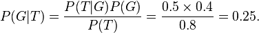
Gibbs Sampling: Gibbs Sampling is one member of a family of algorithms from the Markov Chain Monte Carlo (MCMC) framework [9]. The MCMC algorithms aim to construct a Markov chain that has the target posterior distribution as its stationary distribution. In other words, after a number of iterations of stepping through the chain, sampling from the distribution should converge to be close to sampling from the desired posterior. Gibbs Sampling is based on sampling from conditional distributions of the variables of the posterior.
General Gibbs Sampling Code in Java [and other three languages]- Click here.
Topic Modelling
Topic Modeling Video Lecture: Click here.
Topic Modeling (LDA) Theory: Click here
Topic Modeling (LDA) Technical Report (Implementation): Click here [5].
LDA Gibbs Sampling Code in Java: Click here.
References:
[5] Darling, William M. "A theoretical and practical implementation tutorial on topic modeling and gibbs sampling." Proceedings of the 49th Annual Meeting of the Association for Computational Linguistics: Human Language Technologies. 2011.